Vertical distribution of emissions
Reading the vertical layering of the model
For the vertical distribution of emissions into the model layers, we read the model layer heights from wrfinput.
First, we need some imports:
[1]:
from io import BytesIO

import numpy as np
import pandas as pd
import xarray as xr
import wrf

import matplotlib.pyplot as plt
%matplotlib inline
[2]:
PATH = '/mnt/misc/aether/user/hilboll/prj/2017_cindi-2_wrfchem/wrf/erai-modis/test0007_20170502/WRFV3/run/wrfinput_d01'
The wrfinput_d0X file can be opened with xarray:
[3]:
ds = xr.open_dataset(PATH)
The model layer altitude can be calculated from the base state geopotential PH and perturbation geopotential PHB.
[4]:
var_ph = wrf.getvar(ds._file_obj.ds, 'PH')
var_phb = wrf.getvar(ds._file_obj.ds, 'PHB')
According to the wrf-python source code, the gravitational acceleration is 9.81.
[5]:
z = (var_ph + var_phb) / 9.81
z
[5]:
<xarray.DataArray (bottom_top_stag: 44, south_north: 210, west_east: 210)>
array([[[  0.000000e+00,   0.000000e+00, ...,   0.000000e+00,   2.141231e-01],
        [  0.000000e+00,   0.000000e+00, ...,   0.000000e+00,   0.000000e+00],
        ...,
        [  0.000000e+00,   0.000000e+00, ...,   1.430293e+02,   1.540049e+02],
        [  0.000000e+00,   0.000000e+00, ...,   1.410385e+02,   1.523297e+02]],

       [[  3.351233e+01,   3.350624e+01, ...,   3.359531e+01,   3.380410e+01],
        [  3.350893e+01,   3.350301e+01, ...,   3.357607e+01,   3.356497e+01],
        ...,
        [  3.164389e+01,   3.165490e+01, ...,   1.744284e+02,   1.853996e+02],
        [  3.164697e+01,   3.165774e+01, ...,   1.724226e+02,   1.837137e+02]],

       ...,
       [[  1.946329e+04,   1.946338e+04, ...,   1.948253e+04,   1.948265e+04],
        [  1.946344e+04,   1.946353e+04, ...,   1.948361e+04,   1.948385e+04],
        ...,
        [  1.931028e+04,   1.931158e+04, ...,   1.938800e+04,   1.938841e+04],
        [  1.931019e+04,   1.931152e+04, ...,   1.938659e+04,   1.938711e+04]],

       [[  2.085782e+04,   2.085778e+04, ...,   2.085717e+04,   2.085705e+04],
        [  2.085846e+04,   2.085841e+04, ...,   2.085872e+04,   2.085875e+04],
        ...,
        [  2.074480e+04,   2.074625e+04, ...,   2.080955e+04,   2.080825e+04],
        [  2.074472e+04,   2.074621e+04, ...,   2.080871e+04,   2.080745e+04]]], dtype=float32)
Coordinates:
    XLONG    (south_north, west_east) float32 -12.1618 -12.0042 -11.8463 ...
    XLAT     (south_north, west_east) float32 36.3869 36.4172 36.4471 ...
    Time     datetime64[ns] 2016-09-10
Dimensions without coordinates: bottom_top_stag, south_north, west_east
This yields altitudes on the staggered grid, i.e., at the layer interfaces.
In order to get altitude above ground, we need to subtract the topography height HGT:
[6]:
h_surf = wrf.getvar(ds._file_obj.ds, 'HGT')
h_surf
[6]:
<xarray.DataArray 'HGT' (south_north: 210, west_east: 210)>
array([[   0.      ,    0.      ,    0.      , ...,    0.      ,    0.      ,
           0.214123],
       [   0.      ,    0.      ,    0.      , ...,    0.      ,    0.      ,
           0.      ],
       [   0.      ,    0.      ,    0.      , ...,   15.347553,   10.880167,
           0.      ],
       ...,
       [   0.      ,    0.      ,    0.      , ...,  111.483315,  117.51693 ,
         142.629883],
       [   0.      ,    0.      ,    0.      , ...,  143.721802,  143.029327,
         154.004944],
       [   0.      ,    0.      ,    0.      , ...,  137.794724,  141.038513,
         152.329697]], dtype=float32)
Coordinates:
    XLONG    (south_north, west_east) float32 -12.1618 -12.0042 -11.8463 ...
    XLAT     (south_north, west_east) float32 36.3869 36.4172 36.4471 ...
    Time     datetime64[ns] 2016-09-10
Dimensions without coordinates: south_north, west_east
Attributes:
    FieldType:    104
    MemoryOrder:  XY
    description:  Terrain Height
    units:        m
    stagger:
    coordinates:  XLONG XLAT XTIME
    projection:   LambertConformal(stand_lon=4.927000045776367, moad_cen_lat=...
[7]:
h = z - h_surf
h
[7]:
<xarray.DataArray (bottom_top_stag: 44, south_north: 210, west_east: 210)>
array([[[     0.      ,      0.      , ...,      0.      ,      0.      ],
        [     0.      ,      0.      , ...,      0.      ,      0.      ],
        ...,
        [     0.      ,      0.      , ...,      0.      ,      0.      ],
        [     0.      ,      0.      , ...,      0.      ,      0.      ]],

       [[    33.512325,     33.506245, ...,     33.595314,     33.589973],
        [    33.508926,     33.503006, ...,     33.576065,     33.564968],
        ...,
        [    31.64389 ,     31.654903, ...,     31.399033,     31.394699],
        [    31.646967,     31.657743, ...,     31.384064,     31.384033]],

       ...,
       [[ 19463.285156,  19463.378906, ...,  19482.527344,  19482.4375  ],
        [ 19463.443359,  19463.529297, ...,  19483.611328,  19483.853516],
        ...,
        [ 19310.28125 ,  19311.576172, ...,  19244.974609,  19234.408203],
        [ 19310.191406,  19311.523438, ...,  19245.554688,  19234.783203]],

       [[ 20857.824219,  20857.777344, ...,  20857.173828,  20856.833984],
        [ 20858.458984,  20858.410156, ...,  20858.720703,  20858.753906],
        ...,
        [ 20744.802734,  20746.253906, ...,  20666.517578,  20654.246094],
        [ 20744.716797,  20746.210938, ...,  20667.666016,  20655.123047]]], dtype=float32)
Coordinates:
    XLONG    (south_north, west_east) float32 -12.1618 -12.0042 -11.8463 ...
    XLAT     (south_north, west_east) float32 36.3869 36.4172 36.4471 ...
    Time     datetime64[ns] 2016-09-10
Dimensions without coordinates: bottom_top_stag, south_north, west_east
And indeed, we can see that the lowest level of this new array is indeed 0.0 everywhere:
[8]:
h[0].max().values
[8]:
array(0.0001220703125)
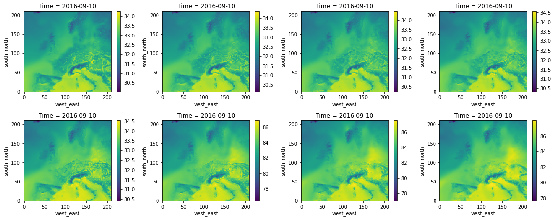
How variable is the layer thickness?
[9]:
delta_h = h[1:] - h[:-1]
fig, axs = plt.subplots(nrows=2, ncols=4, figsize=(40/2.54, 16/2.54))

for i in range(8):
    _ = delta_h[i].plot(ax=axs.ravel()[i])
fig.tight_layout()
Defining the vertical distribution of emission sources (here: from EMEP)
The definition of the vertical levels can be found in Table S3 in Simpson et al. (2012):
[10]:
z_emep = [0., 92., 184., 324., 522., 781., 1106]
zmin_emep, zmax_emep = z_emep[:-1], z_emep[1:]
df_emep = pd.DataFrame()
df_emep['z_min'] = zmin_emep
df_emep['z_max'] = zmax_emep
df_emep['SNAP1'] = [0., 0., .15, .4, .3, .15]
df_emep['SNAP2'] = [1., 0., 0., 0., 0., 0.]
df_emep['SNAP3'] = [.1, .1, .15, .3, .3, .05]
df_emep['SNAP4'] = [.9, .1, 0., 0., 0., 0.]
df_emep['SNAP5'] = [.9, .1, 0., 0., 0., 0.]
df_emep['SNAP6'] = [1., 0., 0., 0., 0., 0.]
df_emep['SNAP7'] = [1., 0., 0., 0., 0., 0.]
df_emep['SNAP8'] = [1., 0., 0., 0., 0., 0.]
df_emep['SNAP9'] = [.1, .15, .4, .35, .0, .0]
df_emep['SNAP10'] = [1., 0., 0., 0., 0., 0.]

assert (df_emep[[c for c in df_emep.columns if c.startswith('SNAP')]].sum() == 1.).all()

df_emep
[10]:
| z_min | z_max | SNAP1 | SNAP2 | SNAP3 | SNAP4 | SNAP5 | SNAP6 | SNAP7 | SNAP8 | SNAP9 | SNAP10 | |
|---|---|---|---|---|---|---|---|---|---|---|---|---|
| 0 | 0.0 | 92.0 | 0.00 | 1.0 | 0.10 | 0.9 | 0.9 | 1.0 | 1.0 | 1.0 | 0.10 | 1.0 |
| 1 | 92.0 | 184.0 | 0.00 | 0.0 | 0.10 | 0.1 | 0.1 | 0.0 | 0.0 | 0.0 | 0.15 | 0.0 |
| 2 | 184.0 | 324.0 | 0.15 | 0.0 | 0.15 | 0.0 | 0.0 | 0.0 | 0.0 | 0.0 | 0.40 | 0.0 |
| 3 | 324.0 | 522.0 | 0.40 | 0.0 | 0.30 | 0.0 | 0.0 | 0.0 | 0.0 | 0.0 | 0.35 | 0.0 |
| 4 | 522.0 | 781.0 | 0.30 | 0.0 | 0.30 | 0.0 | 0.0 | 0.0 | 0.0 | 0.0 | 0.00 | 0.0 |
| 5 | 781.0 | 1106.0 | 0.15 | 0.0 | 0.05 | 0.0 | 0.0 | 0.0 | 0.0 | 0.0 | 0.00 | 0.0 |
Calculating weighting factors per model level
We calculate a matrix of weighting factors to translate the vertical layering of the emission sources to the vertical model layers.
[11]:
model_layer = range(h.shape[0] - 1)
emis_layer = df_emep.index

factor = np.zeros((len(emis_layer), ) + (h.shape[0] - 1, ) + h.shape[1:])

for ml in model_layer:
    for el in emis_layer:
        if h[ml].values.min() > df_emep['z_max'].max():
            break
        upper = np.minimum(h[ml + 1].values, df_emep['z_max'].iloc[el])
        lower = np.maximum(h[ml].values, df_emep['z_min'].iloc[el])
        overlap = np.maximum(upper - lower, 0.)
        factor[el, ml] = overlap / (df_emep['z_max'].iloc[el] - df_emep['z_min'].iloc[el])

assert np.allclose(factor.sum(axis=0).sum(axis=0), emis_layer.max() + 1)
[12]:
for ml in model_layer:
    print(factor[:, ml, 105, 105])
[ 0.35342324  0.          0.          0.          0.          0.        ]
[ 0.35641032  0.          0.          0.          0.          0.        ]
[ 0.29016644  0.06922523  0.          0.          0.          0.        ]
[ 0.          0.36234939  0.          0.          0.          0.        ]
[ 0.          0.36511281  0.          0.          0.          0.        ]
[ 0.          0.20331259  0.47045213  0.          0.          0.        ]
[ 0.          0.          0.52954787  0.05595537  0.          0.        ]
[ 0.          0.          0.          0.43271014  0.          0.        ]
[ 0.          0.          0.          0.43609294  0.          0.        ]
[ 0.          0.          0.          0.07524155  0.27847701  0.        ]
[ 0.          0.          0.          0.          0.33858463  0.        ]
[ 0.          0.          0.          0.          0.34118322  0.        ]
[ 0.          0.          0.          0.          0.04175512  0.24073844]
[ 0.          0.          0.          0.          0.          0.27625018]
[ 0.          0.          0.          0.          0.          0.27858341]
[ 0.          0.          0.          0.          0.          0.20442796]
[ 0.  0.  0.  0.  0.  0.]
[ 0.  0.  0.  0.  0.  0.]
[ 0.  0.  0.  0.  0.  0.]
[ 0.  0.  0.  0.  0.  0.]
[ 0.  0.  0.  0.  0.  0.]
[ 0.  0.  0.  0.  0.  0.]
[ 0.  0.  0.  0.  0.  0.]
[ 0.  0.  0.  0.  0.  0.]
[ 0.  0.  0.  0.  0.  0.]
[ 0.  0.  0.  0.  0.  0.]
[ 0.  0.  0.  0.  0.  0.]
[ 0.  0.  0.  0.  0.  0.]
[ 0.  0.  0.  0.  0.  0.]
[ 0.  0.  0.  0.  0.  0.]
[ 0.  0.  0.  0.  0.  0.]
[ 0.  0.  0.  0.  0.  0.]
[ 0.  0.  0.  0.  0.  0.]
[ 0.  0.  0.  0.  0.  0.]
[ 0.  0.  0.  0.  0.  0.]
[ 0.  0.  0.  0.  0.  0.]
[ 0.  0.  0.  0.  0.  0.]
[ 0.  0.  0.  0.  0.  0.]
[ 0.  0.  0.  0.  0.  0.]
[ 0.  0.  0.  0.  0.  0.]
[ 0.  0.  0.  0.  0.  0.]
[ 0.  0.  0.  0.  0.  0.]
[ 0.  0.  0.  0.  0.  0.]
Applying weighting factors to individual emission sources
Before applying these weighting factors to the individual emission sources, we transpose the weights array in order to speed up lookups of the transformation matrix:
[13]:
factor = factor.transpose(2, 3, 1, 0)
Now, calculating the array of weights per model-layer for a list of emission sources becomes simple:
[14]:
weights_emis = df_emep['SNAP3'].values
ix_geoloc_x, ix_geoloc_y = [0, 1], [1, 2]
np.dot(factor[ix_geoloc_x, ix_geoloc_y], weights_emis)
[14]:
array([[ 0.03641983,  0.03650749,  0.03659634,  0.03668413,  0.03676799,
         0.09126583,  0.09823736,  0.13056395,  0.1315696 ,  0.10501251,
         0.10224079,  0.10313171,  0.01815757,  0.01394153,  0.01406434,
         0.00883902,  0.        ,  0.        ,  0.        ,  0.        ,
         0.        ,  0.        ,  0.        ,  0.        ,  0.        ,
         0.        ,  0.        ,  0.        ,  0.        ,  0.        ,
         0.        ,  0.        ,  0.        ,  0.        ,  0.        ,
         0.        ,  0.        ,  0.        ,  0.        ,  0.        ,
         0.        ,  0.        ,  0.        ],
       [ 0.03640791,  0.03649765,  0.03658518,  0.03667282,  0.03675723,
         0.09124096,  0.09818155,  0.13055235,  0.13155804,  0.10504133,
         0.10223365,  0.10313412,  0.01827613,  0.01394473,  0.01406889,
         0.00884745,  0.        ,  0.        ,  0.        ,  0.        ,
         0.        ,  0.        ,  0.        ,  0.        ,  0.        ,
         0.        ,  0.        ,  0.        ,  0.        ,  0.        ,
         0.        ,  0.        ,  0.        ,  0.        ,  0.        ,
         0.        ,  0.        ,  0.        ,  0.        ,  0.        ,
         0.        ,  0.        ,  0.        ]])